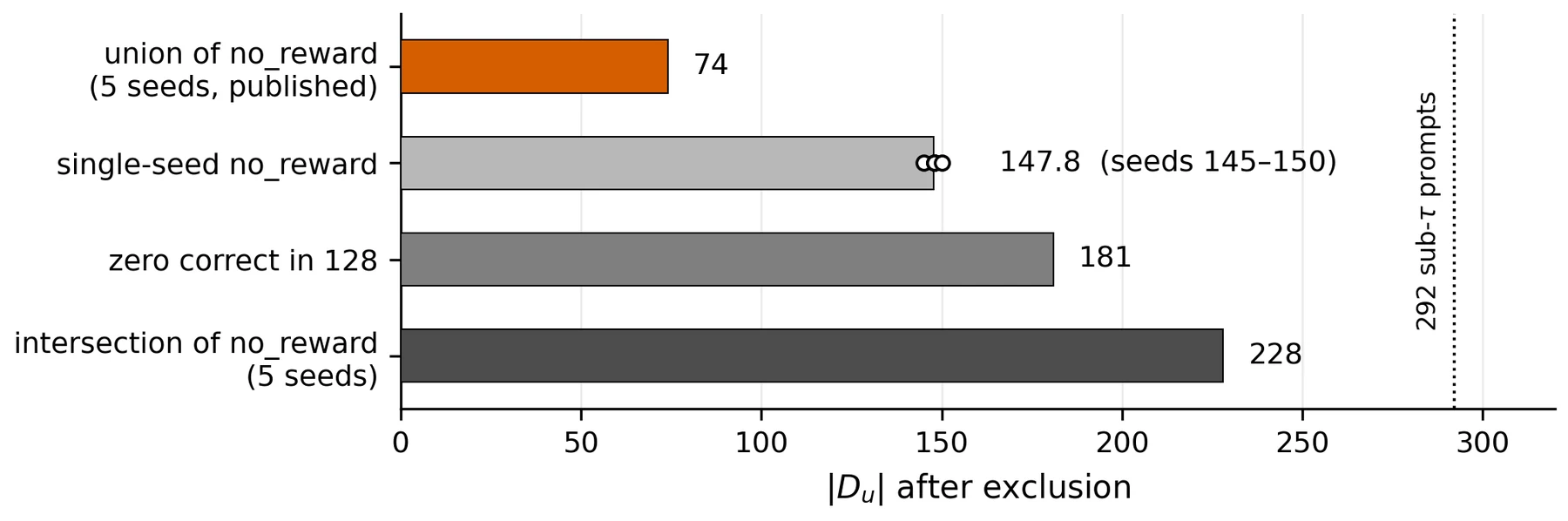
The same 292 candidate hard prompts, four ways of building the “unlearnable” set. Changing only how the five training seeds are combined moves the set from 74 to 228 prompts, while any single seed on its own gives 145–150. The label depends more on the aggregation rule than on which model was trained.
Overview
Reinforcement learning with verifiable rewards (RLVR) is a central tool for improving reasoning in post-training. Recent work reports that some hard prompts stay “unlearnable”: they occasionally produce a correct solution but barely improve during training, which has been linked to low gradient similarity and a possible representation failure. We revisit this phenomenon and ask a prior question: is the set of prompts used to support the claim measured reliably?
Difficulty labels are estimated from a limited number of sampled responses, and combining them across seeds can change which prompts are selected rather than simply reduce noise.
Key findings:
Slow, not static: the prompts labeled unlearnable improve at roughly one third of the learnable rate. The slow-learning effect is real, but literal non-learning is not.
The set depends on the rule: the same candidates give 74 prompts under the published five-seed rule and 228 under an alternative aggregation. Resampling a single checkpoint reproduces about 81% of the apparent cross-seed disagreement.
Budgets can be computed: 8–16 rollouts per prompt give only 0.63–0.73 agreement between repeated labels, and 0.90 needs a projected 242. Our sampling-budget model predicted two budgets before they were measured, and both measurements landed inside the frozen intervals.
The gradient gap shrinks: hard prompts have fewer correct rollouts to average. Matching that count cuts the easy-to-unlearnable gradient-similarity ratio from 2.327× to 1.539×, weakening the evidence without eliminating it.
The slow-learning phenomenon survives our reanalysis, but both the prompts used to define it and the evidence used to explain it require more careful measurement.
Motivation
Prompt difficulty has become an operational quantity in RLVR. Methods use a model's empirical success rate to decide which prompts to replay, filter, route, reweight, or give extra training effort, and difficulty is also used to probe the limits of RLVR itself. Most strikingly, Chen et al. (2026) identified hard prompts that occasionally succeed yet barely improve, called them unlearnable, and connected their behavior to lower within-group gradient similarity.
All of these uses depend on identifying hard prompts reliably. Difficulty is estimated from sampled responses, so the same prompt can land on either side of a threshold across repeated evaluations even when the model is unchanged. We treat the aggregation rule and the rollout budget as part of the measurement, and ask when a prompt-level trainability label is stable enough to support a scientific claim.
Setup
We reproduce the unlearnability study of Chen et al. (2026) and keep its published cohorts, threshold, and verifier.
Component
Configuration
Model
Qwen2.5-0.5B trained with GRPO, G = 8 rollouts per prompt, five independent seeds.
Data
1,023 prompts from MATH; the original answer verifier, unmodified.
Cohorts
The published easy, learnable, and unlearnable groups; difficulty threshold τ = 0.1. Du denotes the set produced by the published unlearnability construction.
Set membership
N = 128 evaluation rollouts per prompt; independent sets compared by Jaccard similarity.
Gradients
N = 200 initial-policy rollouts; each prompt-level gradient averages its correct rollouts.
Uncertainty
95% bootstrap intervals, resampling prompts at the level appropriate to each statistic.
Our run is not a byte-for-byte rerun. The key difference is a 1,024-token generation cap instead of the original 5,120, which we test directly on the evaluation side; the full constant-by-constant audit is below.
“Unlearnable” Prompts Do Learn, Slowly
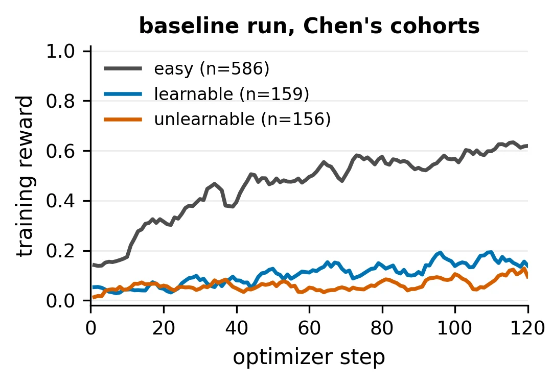
Training reward for the published easy, learnable, and unlearnable cohorts. The separation is present; the flatness is not.
The three published groups stay clearly separated throughout training, but the Du group is not flat. Reward slopes per 100 optimizer steps:
+0.380easy
+0.112learnable
+0.042Du [+0.026, +0.059]
The Du interval excludes zero: these prompts improve at roughly one third of the learnable rate while staying at a much lower reward level.
We use the slope, not the terminal reward, because GRPO drops a prompt from the update once its sampled rewards have zero variance, so the prompts still active late in training are not the same prompts as early on. Throughout, “unlearnable” refers to the published label, not to a claim that these prompts cannot improve.
The Aggregation Rule Changes the Set
To separate training variation from the aggregation rule, we fix a common candidate pool: evaluating all 1,023 prompts 128 times on one reference checkpoint leaves 292 prompts at or below τ = 0.1. From these same candidates:
the published rule, which drops a prompt marked no_reward in any of the five runs, keeps 74;
dropping a prompt only if it is no_reward in all five runs keeps 228;
each training seed on its own keeps 145–150 (mean 147.8);
requiring zero correct responses in the 128-response evaluation keeps 181.
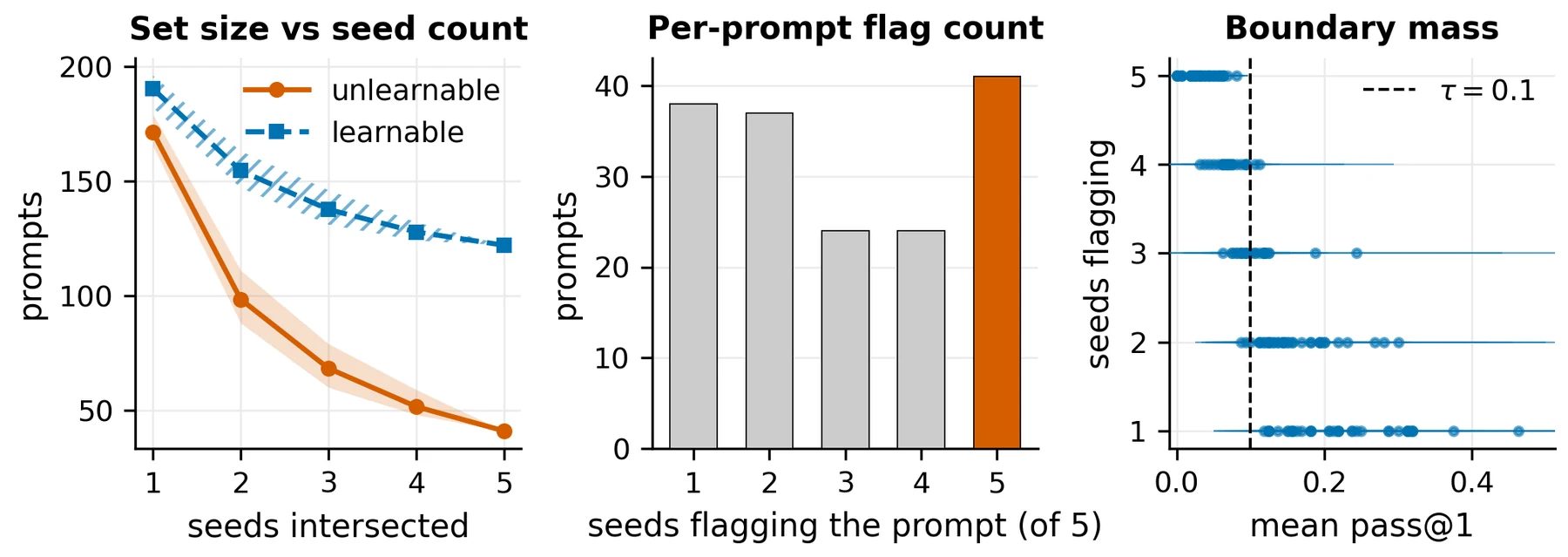
Left: set size keeps falling as more seeds are combined instead of settling. Middle: many prompts are flagged by only some seeds. Right: that disagreement is concentrated near τ = 0.1, where one extra success moves a prompt across the threshold.
What fails is the estimator, not the target. For a fixed policy with true success probability p(x), the set Dτ = {x : p(x) ≤ τ} is well defined. But requiring a prompt to be labeled difficult in every independent run means that, as runs are added, only prompts almost guaranteed that label survive, pushing the retained set toward p(x) = 0. The no_reward exclusion then removes exactly those prompts. The procedure does not converge to Dτ; it converges to a degenerate outcome of the aggregation rule. Pooling the same rollouts into one deeper estimate avoids this.
“No reward was observed in training” is not the same as “unsolvable”: of the 218 prompts removed by the no_reward criterion, 116 are solved at least once in a later N = 128 evaluation.
Most of the Disagreement Is Evaluation Noise
To remove training variation entirely, we evaluate the same checkpoint twice, changing only the sampled rollouts. At N = 32 the two evaluations agree at Jaccard 0.798, versus 0.751 across independently trained seeds: resampling one fixed model reproduces about 81% of the apparent cross-seed disagreement. A binomial model of the threshold decision predicts the same-model agreement to within 0.004.
A longer generation cap does not explain the movement either. Re-evaluating all prompts with 5,120 instead of 1,024 tokens cuts truncation from 9.6% to 3.2%, yet the two sets agree at 0.898, no less than two passes at the same cap (0.877).
Table: Key robustness controls.
Control
Comparison
Result
Interpretation
Same-model resampling
fixed checkpoint vs. cross-seed, N = 32
0.798 vs. 0.751
Most apparent cross-seed disagreement can arise from evaluation sampling alone.
Token-cap sensitivity
1,024 vs. 5,120 tokens
0.898 Jaccard
Set movement is no larger than the measured repeatability scale.
Equal-cost allocation
one N = 128 pass vs. 4×32
0.877 vs. 0.791
A deeper estimate is more reproducible at the same rollout cost.
How Many Rollouts Does a Difficulty Label Need?
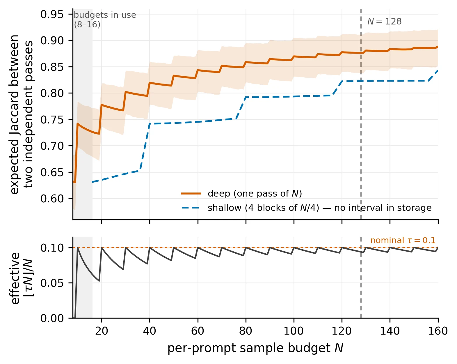
Spend the budget deeply, not in shallow passes. With the same 128 rollouts per prompt, one deep estimate thresholded once agrees across repeats at Jaccard 0.877, while four blocks of 32 intersected agree at only 0.791 (difference +0.086 [+0.038, +0.135]). Both rules use the same effective threshold, ⌊0.1 × 128⌋/128 = ⌊0.1 × 32⌋/32 = 0.09375, so the gain comes from allocation, not from extra compute.
Predicting reproducibility. With N rollouts, a prompt with success probability p is flagged with probability qN(p) = Pr(K ≤ ⌊τN⌋), where K ~ Binomial(N, p). We estimate the distribution F of latent success probabilities from the pooled N = 128 evaluation with the Kiefer–Wolfowitz nonparametric MLE, which accounts for the noise in observed pass rates, and predict the agreement of two independent evaluations:
JN = ∫ qN(p)2 dF(p) / ∫ [2qN(p) − qN(p)2] dF(p)
Predicted agreement versus per-prompt budget N. The sawtooth comes from the integer threshold (bottom), so we report the first budget from which a target stays satisfied.
For Qwen2.5-0.5B on MATH at τ = 0.1:
≈ 40rollouts for 0.80 agreement
242projected for 0.90
2,111projected for 0.95
The 0.90 and 0.95 budgets lie beyond the N = 128 fitting range. These numbers depend on how many prompts sit near the threshold, so they do not transfer to other models, datasets, or thresholds. What transfers is the procedure for computing them.
Table: Predicted Jaccard agreement at representative budgets (deep, single-pass rule).
N rollouts per prompt
8
16
32
64
128
256
512
Predicted Jaccard
0.6322
0.7265
0.7998
0.8413
0.8759
0.9022
0.9171
The Budget Model Predicts Unmeasured Budgets
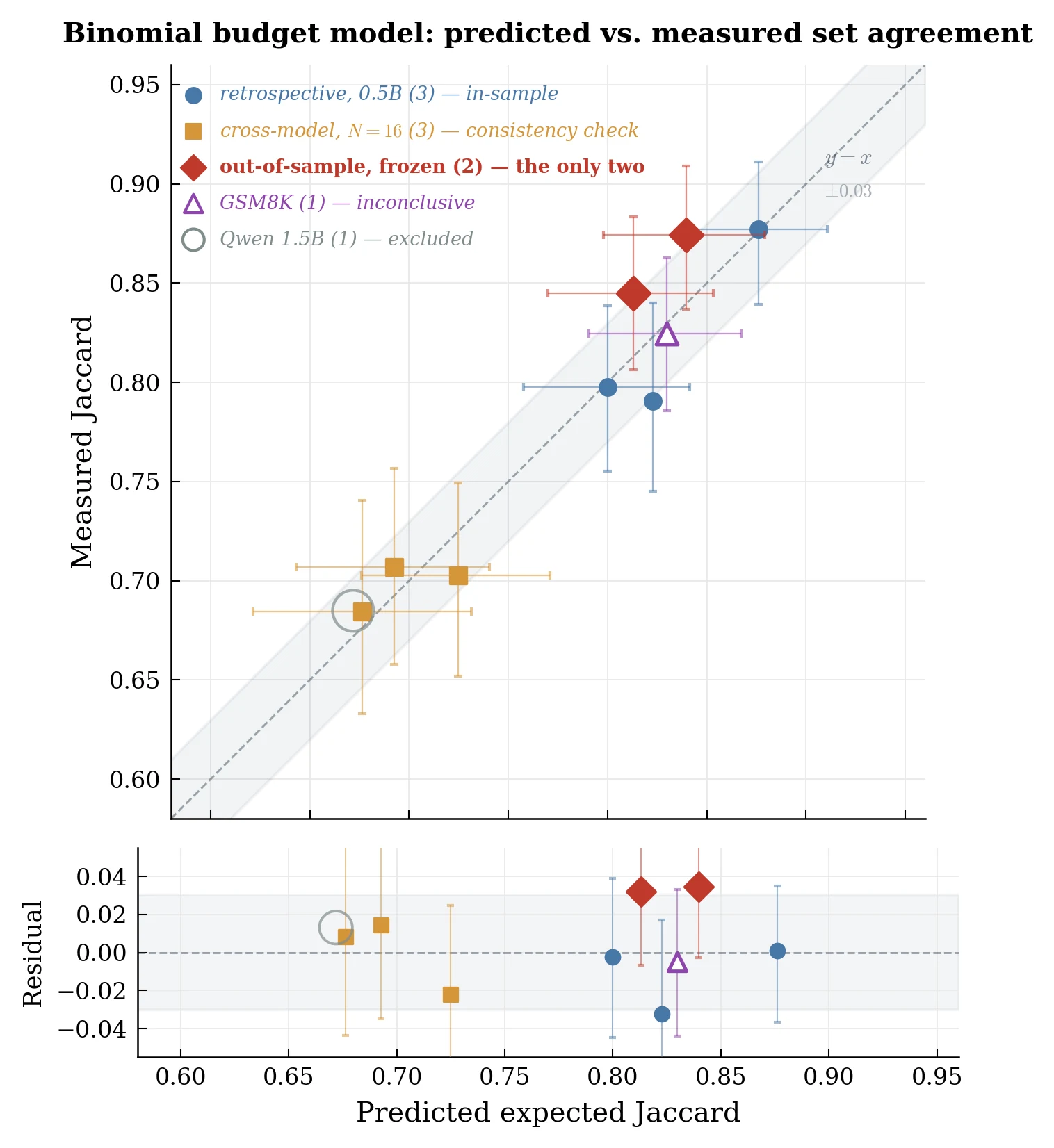
Predicted versus measured agreement. Filled diamonds are the two prospectively frozen predictions; the Qwen2.5-1.5B point is excluded from validation.
We froze and timestamped predictions for two budgets that had not yet been measured, then generated 212,784 new responses:
Budget
Frozen prediction
Measured
N = 40
0.8131 [0.7699, 0.8533]
0.8450 [0.8063, 0.8833]
N = 64
0.8397 [0.7980, 0.8792]
0.8742 [0.8369, 0.9091]
Both measurements fall inside their frozen intervals. The model underpredicts by about 0.03 in both cases, which is conservative: it recommends slightly more sampling, not less.
Set size alone is not enough. A null model that gives every prompt the same success probability matches the number of flagged prompts by construction but misses the measured Jaccard by 0.19–0.53, while the distributional model misses by only 0.008–0.032. What matters is how prompt probabilities are spread around the threshold.
Table: Retrospective and cross-model consistency checks. Cross-model rows reuse the pass their distribution was estimated from, so they are consistency checks rather than independent validation; the Qwen2.5-1.5B row (greyed) is an excluded diagnostic.
Model / rule
Measured
Predicted
Error
Qwen2.5-0.5B, one pass N = 32
0.7977
0.8000
+0.0023
Qwen2.5-0.5B, one pass N = 128
0.8770
0.8759
−0.0011
Qwen2.5-0.5B, four blocks of 32
0.7906
0.8228
+0.0322
Qwen2.5-0.5B, two blocks of 16
0.7028
0.7248
+0.0220
Llama-3.2-3B, two blocks of 16
0.6844
0.6763
−0.0081
Llama-3.2-3B v2, two blocks of 16
0.7070
0.6926
−0.0144
Qwen2.5-1.5B, two blocks of 16
0.6849
0.6718
−0.0131
The Gradient Gap Shrinks When Sample Count Is Matched
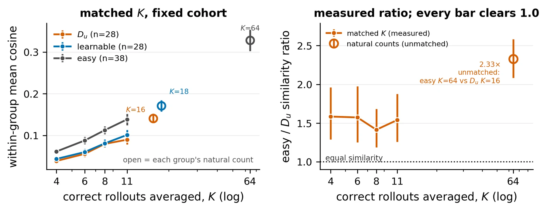
The gradient explanation compares how similar per-prompt gradients are within each group, but each prompt-level gradient averages its correct rollouts, and hard prompts have far fewer: in the N = 200 cohort, a median of 8 for Du versus 65 for easy prompts.
2.327×easy / Du ratio, unmatched
1.539×matched at K = 11 [1.26, 1.88]
48.9%of the log-gap removed [29.3, 71.2]
Every matched level (K = 4, 6, 8, 11) lies below the unmatched ratio and above one, so matching weakens the separation substantially without eliminating it. Matching also selects: at K = 11 only 28 of the 71 Du prompts remain, and they are the easier ones, so this shows sensitivity to sample count, not a corrected full-cohort estimate.
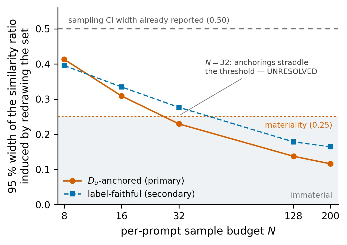
Set uncertainty propagates downstream: at N = 8 it alone adds a 95% interval width of 0.41 to the gradient ratio, falling to 0.14 by N = 128.
Two Simple Optimization Explanations Do Not Hold
Exposure starvation. With G = 8, a prompt only updates the policy when its sampled rewards differ. Du prompts contribute on 2.14 steps per run, versus 3.13 for learnable and 5.26 for easy prompts. The gap is real, but none of the 156 prompts in the exposure cohort is fully starved across all five runs, and 22.4% receive at least the learnable group's mean exposure while still improving slowly.
GRPO normalization. If reward-std normalization suppressed hard prompts, Du updates would be smaller. The opposite holds: when a prompt does contribute, the mean 1/σ scale is 2.836 for Du and 2.426 for easy prompts, about 17% larger. The asymmetry is in how often an update forms, not in its scale.
Content starvation, where rewarded trajectories carry weak learning signal, remains possible; we cannot test it because the training-time responses were not stored. The cause of the slow-learning effect is still unresolved.
An Unstable Label Does Not Necessarily Mean Unstable Training
Does a noisy difficulty rule make difficulty-aware RLVR ineffective? We train five seeds under two neighboring constructions that remove very different amounts of usable training signal, 5.0% versus 27.6% after GRPO's zero-variance filter, alongside size-matched random-removal controls. The resulting models differ by less than one held-out accuracy point. The experiment cannot resolve effects that small, so this is not evidence of equivalence, but it bounds our claim: a large change in the reported set need not produce an equally large change in training. Our conclusion is about measurement and inference, not a claim that every method using noisy difficulty signals must fail.
Replication Audit
We audited the effective configuration from the actual training and evaluation paths: of 47 effective constants, 30 match the original and the 17 below differ. The generation cap matters most, since it affects hard prompts more than easy ones; its evaluation-side effect is tested above, but our training-dependent magnitudes should not be read as an exact reproduction of the original configuration. All runs used a single NVIDIA RTX 3090 Ti (24 GB).
Configuration constant
Ours
Original
Training
Dataset name
simplelr_qwen_level1to4_sub1k
simplelr_qwen_level1to4
Maximum response length
1,024
5,120
Train batch size
32
256
PPO mini-batch size
16
64
PPO micro-batch size
2
32
Log-probability micro-batch size
4
128
Micro rollout batch size
128
1,024
Tensor parallelism
1
2
GPUs per node
1
4
Rollout GPU memory utilization
0.45
0.75
Total epochs
12
50
Save frequency
40
20
Test frequency
100,000
5
Validation batch size
200
1,000
Evaluation
Test data
Training subset used here
Original test split
Maximum generation length
1,024
5,120
GPU memory utilization
0.60
0.75
Conclusion
We revisited the unlearnability phenomenon in RLVR and found a more nuanced result. The affected prompts improve at roughly one third of the learnable rate rather than not at all, but the prompts used to define them are far less stable than the effect itself. The published aggregation rule does not consistently recover a fixed-threshold set, and finite-sample evaluation explains much of the apparent disagreement across training seeds.
We provide a way to determine how much evaluation reproducible difficulty assignment requires, and validate its predictions at previously unmeasured budgets. The gradient-similarity difference proposed to explain unlearnability shrinks substantially when estimator sample count is matched, although a residual gap remains. The lesson is not that unlearnability disappears, but that low-budget difficulty labels are unreliable for classifying individual prompts as “unlearnable,” or for supporting mechanistic claims built on that classification.
BibTeX
@inproceedings{chakma2026unlearnable,
    title={Unlearnable, or Unmeasured? On the Reliability of Difficulty Labels in RLVR},
    author={Chakma, Chandak and Sakib, Syed Nazmus and Haque, Nafiul and
            Arman, Shifat E.},
    booktitle={NeurIPS 2026 Workshop: Transitioning from Pre-Training to Post-Training},
    year={2026}
}